How to Master VLOOKUP, HLOOKUP, XLOOKUP, LEFT & RIGHT in Excel

Finding information in a large Excel sheet can take a lot of time. You may have hundreds of names, IDs, prices, or marks. Searching for each value by hand is slow and can also cause mistakes. But Excel has simple functions that can do this work for you.

In this guide, you will learn VLOOKUP, HLOOKUP, and XLOOKUP with easy examples. You will also learn how LEFT and RIGHT can help you work with text. These functions are useful for students, teachers, office workers, and business users. So, let’s learn how each function works and when you should use it.

What Are Lookup Functions in Excel?

Lookup functions help you find data in a table. You give Excel a value to search for. Excel then finds that value and returns the related information.

For example, you may have a student ID and want to find the student’s marks. Instead of checking every row, you can use a lookup formula. As a result, Excel can find the answer in seconds.

The three main lookup functions are VLOOKUP, HLOOKUP, and XLOOKUP. Each one works differently, so it is important to understand the differences.

VLOOKUP in Excel

What Does VLOOKUP Do?

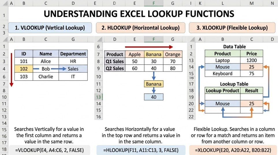
VLOOKUP means Vertical Lookup. It searches for a value in the first column of a table. Then, it returns a value from another column in the same row.

For example, you may have student IDs in column A, names in column B, and marks in column C. If you know the student ID, VLOOKUP can find the marks for you.

The basic formula is:

=VLOOKUP(lookup_value, table_array, column_index_num, [range_lookup])

The lookup value is the value you want to find. The table array is the data range. The column index tells Excel which column contains the result. The last part controls exact or approximate matching.

Simple VLOOKUP Example

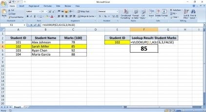
Suppose your table looks like this:

Student ID	Name	Marks
101	Ali	78
102	Sara	85
103	Ahmed	91

If cell E2 contains 102, you can use:

=VLOOKUP(E2,A2:C4,3,FALSE)

Excel searches for 102 in the first column. It then returns the mark from the third column. The result is 85.

For an exact result, FALSE is usually the best choice. This is helpful when you search for IDs, codes, or specific names.

HLOOKUP in Excel

What Does HLOOKUP Do?

HLOOKUP means Horizontal Lookup. It is useful when your data is arranged across rows.

This is one of the main differences between VLOOKUP, HLOOKUP, XLOOKUP, and VLOOKUP: VLOOKUP searches down a column, while HLOOKUP searches across the first row.

The basic formula is:

=HLOOKUP(lookup_value, table_array, row_index_num, [range_lookup])

The formula uses a lookup value, table range, row number, and match setting.

Simple HLOOKUP Example

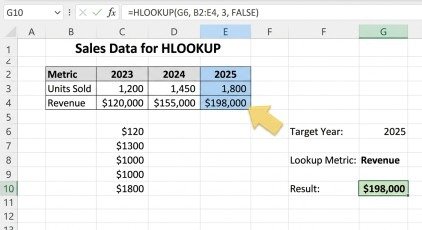
Imagine that years are placed in the first row. Sales values are placed in the rows below.

You can use:

=HLOOKUP(2025,B1:D6,4,FALSE)

Excel looks for 2025 in the first row. Then, it returns the value from the fourth row.

HLOOKUP is useful for horizontal tables. However, it is less flexible when your data layout changes.

XLOOKUP in Excel

What Makes XLOOKUP Different?

XLOOKUP is a newer and more flexible lookup function. It can search vertically or horizontally. It can also return data from a range on either side of the lookup range.

This makes VLOOKUP HLOOKUP XLOOKUP easier to compare. VLOOKUP and HLOOKUP have fixed layouts. XLOOKUP gives you more freedom.

The basic formula is:

=XLOOKUP(lookup_value, lookup_array, return_array, [if_not_found], [match_mode], [search_mode])

The lookup array is where Excel searches. The return array contains the answer. You can also add a message for a missing value.

Simple XLOOKUP Example

Suppose column B contains product names and column A contains prices.

You can use:

=XLOOKUP("Bananas",B2:B4,A2:A4,"Not Found")

Excel searches for Bananas in column B. It then returns the matching price from column A.

If Bananas is not found, Excel displays Not Found.

This is a useful feature because you do not need to count columns like you do with VLOOKUP.

VLOOKUP HLOOKUP XLOOKUP: Main Differences

Choosing the right function becomes easy when you understand how each one searches.

VLOOKUP works best with vertical tables. The lookup value must be in the first column of the selected table.

HLOOKUP works best with horizontal tables. The lookup value must be in the first row.

XLOOKUP is more flexible. It can search in different directions and can return data from a separate range.

The source comparison shows that VLOOKUP searches down, HLOOKUP searches across, while XLOOKUP can work in any direction. It also shows that XLOOKUP has built-in handling for values that are not found.

For modern Excel, XLOOKUP is often a strong choice. However, older Excel versions may not support it. In that case, VLOOKUP or HLOOKUP can still be useful.

LEFT Function in Excel

What Does LEFT Do?

LEFT is a text function. It takes characters from the left side of a text value.

The basic formula is:

=LEFT(text, [num_chars])

For example:

=LEFT("Excel",2)

The result is:

Ex

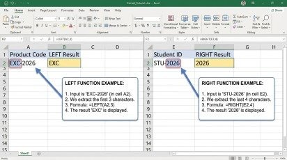
You can also use a cell. If A2 contains EXC-2026, use:

=LEFT(A2,3)

The result will be:

EXC

LEFT is useful when you need the first part of a code, name, or other text.

RIGHT Function in Excel

What Does RIGHT Do?

RIGHT works from the opposite side. It takes characters from the right side of a text value.

The formula is:

=RIGHT(text, [num_chars])

For example:

=RIGHT("Excel",2)

The result is:

el

If A2 contains STU-2026, you can use:

=RIGHT(A2,4)

The result will be:

2026

Therefore, RIGHT is helpful when the information you need is at the end of a text value.

How These Excel Functions Help in Real Work

Learning VLOOKUP HLOOKUP XLOOKUP can make many Excel tasks faster.

A teacher can use lookup formulas to find student marks. A business user can find product prices. An office worker can retrieve employee details. Students can also use these functions when working with large class records.

LEFT and RIGHT are useful for text cleaning. For example, you can use them to extract a year, code, prefix, or part of an ID.

As a result, these functions can reduce manual work and make your spreadsheet easier to manage.

Common Excel Errors

Even a good formula can show an error. So, always check your data when something goes wrong.

#N/A Error

An #N/A error often means that Excel cannot find the value. Check the spelling and make sure the lookup value exists in the selected range.

XLOOKUP lets you add a custom message when a value is missing. For example:

=XLOOKUP(A2,B2:B10,C2:C10,"Not Found")

This gives a clear result instead of only showing an error.

#REF! Error

A #REF! error may appear when the column or row number is outside the selected table.

For example, if your table has four columns, do not ask VLOOKUP to return column 6. Check your table range and column number.

#VALUE! Error

With XLOOKUP, the lookup range and return range should match correctly. If their sizes do not line up, Excel may return a #VALUE! error.

Tips for Better Excel Formulas

Good data makes VLOOKUP HLOOKUP XLOOKUP formulas easier to use.

First, keep your table clean. Use clear headings and avoid unnecessary blank rows.

Next, check your lookup values. Extra spaces or spelling differences can stop Excel from finding a match.

Also, use FALSE when you need an exact match. This is often safer for IDs and codes.

When copying a formula, you can lock a range with $ signs. For example:

=VLOOKUP(A2,$A$2:$D$100,3,FALSE)

The locked range stays the same when you copy the formula.

VLOOKUP HLOOKUP XLOOKUP: Which One Is Best?

The best function depends on your data.

If your lookup value is in the first column, VLOOKUP can be a simple choice. If your lookup value is in the first row, HLOOKUP may be useful.

If you want more flexibility, XLOOKUP is often easier. It can search in different directions and can use a separate return range.

So, do not choose a function only because it is newer. First, look at your table. Then, choose the function that fits your data.

Final Thoughts

Excel becomes much easier when you know the right functions. VLOOKUP HLOOKUP XLOOKUP can help you find data without checking every row or column by hand. VLOOKUP is useful for vertical data, HLOOKUP works with horizontal data, and XLOOKUP gives you more flexibility.

LEFT and RIGHT also make text work easier. They can extract useful parts from IDs, codes, years, and other text.

The best way to learn these functions is to practice them with a small table. Start with one formula. Test the result. Then try a different example.

With regular practice, VLOOKUP HLOOKUP XLOOKUP and the LEFT and RIGHT functions can become simple tools for your daily Excel work.

Frequently Asked Questions

1. What is the main difference between VLOOKUP and HLOOKUP?

VLOOKUP searches vertically in the first column, while HLOOKUP searches horizontally across the first row of a table.

2. Why is XLOOKUP more flexible than VLOOKUP?

XLOOKUP can search in different directions and return data from a separate range, so you do not need to count columns.

3. When should I use VLOOKUP in Excel?

Use VLOOKUP when your lookup value is in the first column and you need to return related data from another column.

4. What is the purpose of LEFT and RIGHT in Excel?

LEFT extracts characters from the beginning of text, while RIGHT extracts characters from the end of a text value.

Meta Description

Learn VLOOKUP, HLOOKUP, XLOOKUP, LEFT and RIGHT in Excel with simple formulas, examples, and easy tips for faster data lookup.